
Introduction
The new Flux language introduced in InfluxDB v2 addresses many InfluxQL language limitations.
Let’s see some of the features now possible using Flux language on time series data : joins, pivots, histograms…
In most topics, real use cases are discussed : joining data when timestamps differ by a few seconds,
simulating outer joins waiting for the new join methods to come (left, right…), building histograms without cumulative data but the difference…
Using SQL data sources in Flux language is not addressed here, this topic deserves a dedicated article : InfluxDB v2, Flux language and SQL databases
- For beginners in the Flux language and used to InfluxQL : InfluxDB - Moving from InfluxQL to Flux language
- The sections of this paper are also summarized in a reference guide/cheat sheet : InfluxDB v2 : Flux language, quick reference guide and cheat sheet
InfluxDB v2, Quick reminders
Output format
It’s important to understand the InfluxDB v2 raw data output format, different than the v1 output format. In the output below, filter is set only on the measurement name, filters on tag keys and on field keys are not applied.
from(bucket: "netdatatsdb/autogen")
 |> range(start: -1d)
 |> filter(fn: (r) => r._measurement == "vpsmetrics")
 |> yield()
table _start _stop _time _value _field _measurement host location
----- -------------------- --------------------- ------------------------------ ------ ------ ------------ ------------ --------
0 2021-02-05T00:00:00Z 2021-02-05T23:59:00Z 2021-02-05T03:00:06.446501067Z 1182 mem vpsmetrics vpsfrsqlpac1 france
0 2021-02-05T00:00:00Z 2021-02-05T23:59:00Z 2021-02-05T03:00:16.604175869Z 817 mem vpsmetrics vpsfrsqlpac1 france
…
1 2021-02-05T00:00:00Z 2021-02-05T23:59:00Z 2021-02-05T03:00:06.446501067Z 62 pcpu vpsmetrics vpsfrsqlpac1 france
1 2021-02-05T00:00:00Z 2021-02-05T23:59:00Z 2021-02-05T03:00:16.604175869Z 66 pcpu vpsmetrics vpsfrsqlpac1 france
…
2 2021-02-05T00:00:00Z 2021-02-05T23:59:00Z 2021-02-05T03:00:07.420674651Z 429 mem vpsmetrics vpsfrsqlpac2 france
2 2021-02-05T00:00:00Z 2021-02-05T23:59:00Z 2021-02-05T03:00:17.176860469Z 464 mem vpsmetrics vpsfrsqlpac2 france
…
3 2021-02-05T00:00:00Z 2021-02-05T23:59:00Z 2021-02-05T03:00:07.420674651Z 29 pcpu vpsmetrics vpsfrsqlpac2 france
3 2021-02-05T00:00:00Z 2021-02-05T23:59:00Z 2021-02-05T03:00:17.176860469Z 32 pcpu vpsmetrics vpsfrsqlpac2 france- A table identifier is applied on each results set.
- Range time is fully described by the columns
_startand_stop. - The measurement name is in the column
_measurement. - The field key and its value are respectively in the columns
_fieldand_value. - Tag keys columns are displayed at the end.
Columns can be removed using the drop or keep functions, we may
not want all the columns in the raw data ouput format.
|> keep(columns: ["_value", "_time"]) |> drop(fn: (column) => column =~ /^_(start|stop)/)Columns are renamed using rename function :
 |> keep(columns: ["_value", "_time"])
 |> rename(columns: {_value: "pcpu", _time: "when"})
Querying data
In this article, Flux queries are executed with one of the 2 following methods :
influxclient command line.- Integrated InfluxDB v2 GUI
https://<host-influxdb>:8086(formerly Chronograf in InfluxDB v1 Tick stack suite).
influx client
$ influx query --file query.fluxTo be able to use influx client, config (url, token, org…) is defined before.
$ export INFLUX_CONFIGS_PATH=/sqlpac/influxdb/srvifx2sqlpac/configs
$ export INFLUX_ACTIVE_NAME=default
/sqlpac/influxdb/srvifx2sqlpac/configs :
[default]
  url = "https://vpsfrsqlpac:8086"
  token = "K2YXbGhIJIjVhL…"
  org = "sqlpac"
  active = true
InfluxDB v2 GUI
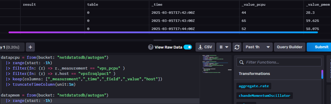
In the InfluxDB GUI : use "View Raw Data" toggle button to display queries raw results sets.
Joins
In the use case, cpu and memory used percentages per host are stored respectively in vps_cpu and
vps_pmem measurements :
_measurement   _time                             _field    _value    host
------------   ------------------------------    ------    ------    ------------
vps_pcpu       2021-03-01T17:22:10.009239717Z    pcpu      63        vpsfrsqlpac1
vps_pcpu       2021-03-01T17:23:10.459116034Z    pcpu      73        vpsfrsqlpac1
vps_pcpu 2021-03-01T17:24:10.938936764Z pcpu 57 vpsfrsqlpac1_measurement _time _field _value host
------------ ------------------------------ ------ ------ ------------
vps_pmem 2021-03-01T17:22:10.095918231Z pmem 26.8 vpsfrsqlpac1
vps_pmem 2021-03-01T17:23:10.575832095Z pmem 29.725 vpsfrsqlpac1
vps_pmem 2021-03-01T17:24:11.011812310Z pmem 22.325 vpsfrsqlpac1Reading the documentation, one may conclude : it is easy to join data with the join function !
datapcpu = from(bucket: "netdatatsdb/autogen")
  |> range(start: -1h)
  |> filter(fn: (r) => r._measurement == "vps_pcpu" )
  |> filter(fn: (r) => r.host == "vpsfrsqlpac1" )
  |> keep(columns: ["_measurement","_time","_field","_value","host"])

datapmem = from(bucket: "netdatatsdb/autogen")
  |> range(start: -1h)
  |> filter(fn: (r) => r._measurement == "vps_pmem" )
  |> filter(fn: (r) => r.host == "vpsfrsqlpac1" )
  |> keep(columns: ["_measurement","_time","_field","_value","host"])

join(
    tables: {pcpu:datapcpu, pmem:datapmem},
    on: ["_time","host"],
    method: "inner"
)
  |> keep(columns: ["_value_pmem", "_value_pcpu", "_time"])
Executing the query : no results ! Why ?
Normalizing irregular timestamps
In real systems, joining on _time columns is always problematic.
The column _time usually stores seconds, milliseconds, microseconds… which are very slightly different to join 2 points.
First solution : use truncateTimeColumn function to normalize irregular timestamps. This function truncates
all _time values to a specified unit. In the above example, _time values are truncated to the minute : join works.
datapcpu = from(bucket: "netdatatsdb/autogen") |> range(start: -1h) |> filter(fn: (r) => r._measurement == "vps_pcpu" ) |> filter(fn: (r) => r.host == "vpsfrsqlpac1" ) |> keep(columns: ["_measurement","_time","_field","_value","host"]) |> truncateTimeColumn(unit:1m) datapmem = from(bucket: "netdatatsdb/autogen") |> range(start: -1h) |> filter(fn: (r) => r._measurement == "vps_pmem" ) |> filter(fn: (r) => r.host == "vpsfrsqlpac1" ) |> keep(columns: ["_measurement","_time","_field","_value","host"]) |> truncateTimeColumn(unit:1m) join( tables: {pcpu:datapcpu, pmem:datapmem}, on: ["_time","host"], method: "inner" ) |> keep(columns: ["_value_pmem", "_value_pcpu", "_time"])_time:time _value_pcpu:float _value_pmem:float ------------------------------ ---------------------------- ---------------------------- 2021-03-01T17:22:00.000000000Z 63 26.8 2021-03-01T17:23:00.000000000Z 73 29.725 2021-03-01T17:24:00.000000000Z 57 22.325
If technically and functionnally acceptable, the aggregateWindow function is another alternative solution.
datapcpu = from(bucket: "netdatatsdb/autogen") |> range(start: -1h) |> filter(fn: (r) => r._measurement == "vps_pcpu" ) |> filter(fn: (r) => r.host == "vpsfrsqlpac1" ) |> keep(columns: ["_measurement","_time","_field","_value","host"]) |> aggregateWindow(every: 1m, fn: mean) datapmem = from(bucket: "netdatatsdb/autogen") |> range(start: -1h) |> filter(fn: (r) => r._measurement == "vps_pmem" ) |> filter(fn: (r) => r.host == "vpsfrsqlpac1" ) |> keep(columns: ["_measurement","_time","_field","_value","host"]) |> aggregateWindow(every: 1m, fn: mean) join( tables: {pcpu:datapcpu, pmem:datapmem}, on: ["_time","host"], method: "inner" ) |> keep(columns: ["_value_pmem", "_value_pcpu", "_time"])_time:time _value_pcpu:float _value_pmem:float ------------------------------ ---------------------------- ---------------------------- 2021-03-01T17:23:00.000000000Z 63 26.8 2021-03-01T17:24:00.000000000Z 73 29.725 2021-03-01T17:25:00.000000000Z 57 22.325
Joins methods and limitations
In the previous use case, join is performed using the inner method.
join(
    tables: {pcpu:datapcpu, pmem:datapmem},
    on: ["_time","host"],
    method: "inner"
)
Only the inner method is currently allowed (v 2.0.4).
In future releases, other joins methods will be gradually implemented : cross, left, right, full.
Another limitation : joins currently must only have two parents. This limit should be also extended in future releases.
How to manage outer joins waiting the other methods to be ready ?
The combination of the aggregateWindow and fill functions is a potential workaround to manage outer joins for the moment.
The fill function replaces the NULL values by a default value, the default value applied will depend on the technical context and desired rendering (charts…).
| Previous value | Fixed value |
|---|---|
|
|
datapcpu = from(bucket: "netdatatsdb/autogen") |> range(start: -1h) |> filter(fn: (r) => r._measurement == "vps_pcpu" ) |> filter(fn: (r) => r.host == "vpsfrsqlpac1" ) |> keep(columns: ["_measurement","_time","_field","_value","host"]) |> aggregateWindow(every: 1m, fn: mean) |> fill(column: "_value", value: 0.0) datapmem = from(bucket: "netdatatsdb/autogen") |> range(start: -1h) |> filter(fn: (r) => r._measurement == "vps_pmem" ) |> filter(fn: (r) => r.host == "vpsfrsqlpac1" ) |> keep(columns: ["_measurement","_time","_field","_value","host"]) |> aggregateWindow(every: 1m, fn: mean) |> fill(column: "_value", value: 0.0) join( tables: {pcpu:datapcpu, pmem:datapmem}, on: ["_time","host"] ) |> keep(columns: ["_value_pmem", "_value_pcpu", "_time"])_time:time _value_pcpu:float _value_pmem:float ------------------------------ ---------------------------- ---------------------------- 2021-03-01T18:23:00.000000000Z 76 26 2021-03-01T18:24:00.000000000Z 63 24.65 2021-03-01T18:25:00.000000000Z 54 0.0 2021-03-01T18:26:00.000000000Z 69 0.0 2021-03-01T18:27:00.000000000Z 61 0.0 2021-03-01T18:28:00.000000000Z 79 23.4 2021-03-01T18:29:00.000000000Z 65 21.8
Pivot
Default output format is really not easy for some specific further processings (writing to another measurement, to a SQL database…).
from(bucket: "netdatatsdb/autogen") |> range(start: -1h) |> filter(fn: (r) => r._measurement == "vps_pcpumem" and r.host == "vpsfrsqlpac1" ) |> keep(columns: ["_measurement","_time","_field","_value","host"])Table: keys: [_field, _measurement, host] _field:string _measurement:string host:string _time:time _value:float ------------------ ---------------------- ---------------------- ------------------------------ ------------------- mem vps_pcpumem vpsfrsqlpac1 2021-03-01T18:50:46.919579473Z 1055 mem vps_pcpumem vpsfrsqlpac1 2021-03-01T18:51:47.359821389Z 1069 … … … … … Table: keys: [_field, _measurement, host] _field:string _measurement:string host:string _time:time _value:float ------------------ ---------------------- ---------------------- ------------------------------ ------------------- pcpu vps_pcpumem vpsfrsqlpac1 2021-03-01T18:50:46.919579473Z 68 pcpu vps_pcpumem vpsfrsqlpac1 2021-03-01T18:51:47.359821389Z 57 … … … … …
Pivoting data to format output was a major missing feature in InfluxQL. Feature ready and easy to use in Flux language :
from(bucket: "netdatatsdb/autogen") |> range(start: -1h) |> filter(fn: (r) => r._measurement == "vps_pcpumem" and r.host == "vpsfrsqlpac1") |> keep(columns: ["_measurement","_time","_field","_value","host"]) |> pivot( rowKey:["_time"], columnKey: ["_field"], valueColumn: "_value" )Table: keys: [_measurement, host] _measurement:string host:string _time:time mem:float pcpu:float ---------------------- --------------- ------------------------------ ------------------- --------------------- vps_pcpumem vpsfrsqlpac1 2021-03-01T18:50:46.919579473Z 1055 68 vps_pcpumem vpsfrsqlpac1 2021-03-01T18:51:47.359821389Z 1069 57 … … … … …
Like joins, if needed use the truncateTimeColumn function to normalize timestamps.
Use schema.fieldsAsCols() shortcut function when pivoting data only on time/_field :
import "influxdata/influxdb/schema"

from(bucket: "netdatatsdb/autogen")
  |> range(start: -1h)
  |> filter(fn: (r) => r._measurement == "vps_pcpumem" and
                       r.host == "vpsfrsqlpac1" )
  |> keep(columns: ["_measurement","_time","_field","_value","host"])
  |> schema.fieldsAsCols()
Histograms
Producing histograms by a query is made simple in the Flux language with histogram and linearBins functions.
linearBins function eases the creation of the list of linearly separated floats ([0.0,5.0,10.0,15.0,…]).
from(bucket:"netdatatsdb/autogen") |> range(start: -1d) |> filter(fn: (r) => r._measurement == "vps_pcpumem" and r.host == "vpsfrsqlpac1" and r._field == "pcpu" ) |> histogram( bins: linearBins(start: 0.0, width: 5.0, count: 21, infinity: false) ) |> keep(columns: ["le","_value"])le:float _value:float ---------------------------- ---------------------------- 0 0 5 0 10 0 15 0 20 0 25 0 30 0 35 0 40 42 45 206 50 389 55 547 60 716 65 910 70 1085 75 1260 80 1427 85 1427 90 1427 95 1427 100 1427
A column named le (less or equals) is automatically created, in the _value column data are cumulative.
Apply the difference function to cancel the cumulative mode and thus build a typical histogram
|> histogram( bins: linearBins(start: 0.0, width: 5.0, count: 21, infinity: false) ) |> difference() |> keep(columns: ["le","_value"])le:float _value:float ---------------------------- ---------------------------- 5 0 10 0 15 0 20 0 25 0 30 0 35 0 40 42 45 161 50 183 55 156 60 172 65 195 70 175 75 175 80 169 85 0 90 0 95 0 100 0
Logarithmic mode is performed with logarithmicBins function.
  |> histogram(
       bins: logarithmicBins(start: 1.0, factor: 2.0, count: 10,
                           infinity: false)
histogram function is of interest when we need to build histograms by programming for further processing.
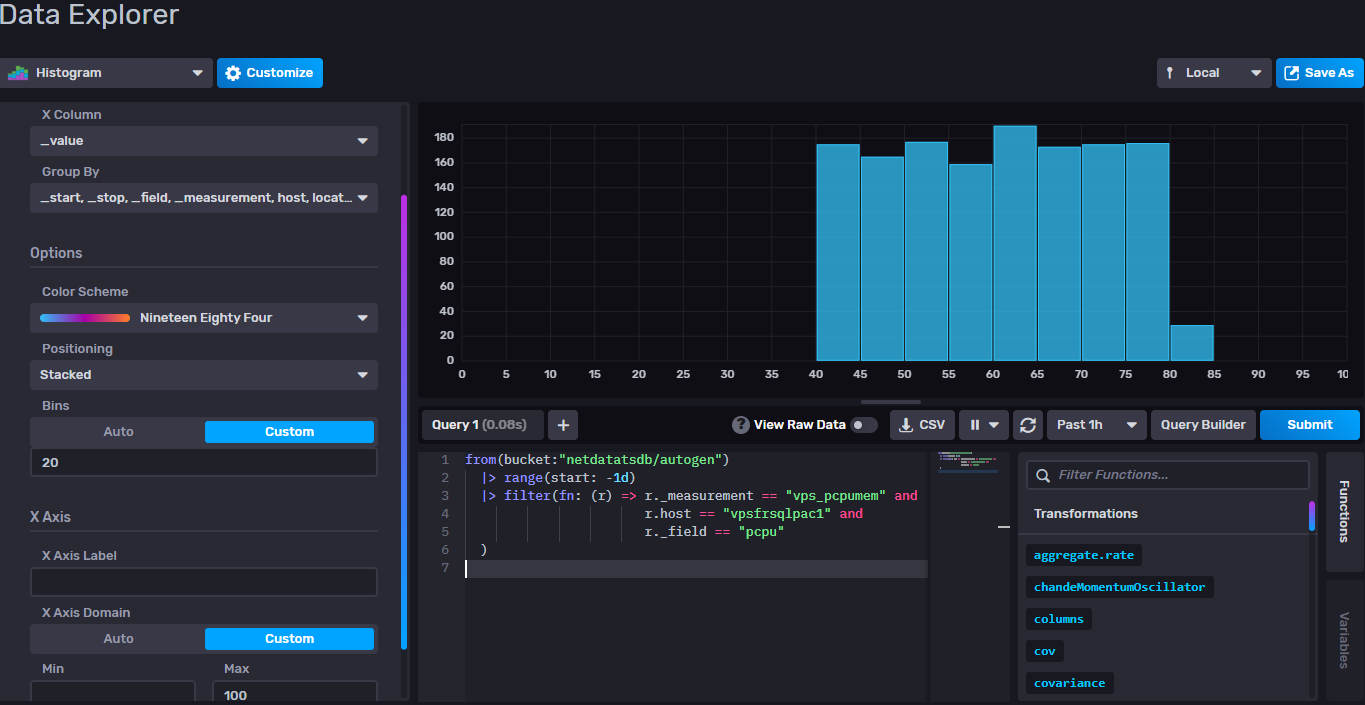
InfluxDB GUI or Grafana does not need the histogram function.
In InfluxDB GUI, to visualize an histogram :
- The query source without
histogramfunction call is used.from(bucket:"netdatatsdb/autogen") |> range(start: -1d) |> filter(fn: (r) => r._measurement == "vps_pcpumem" and r.host == "vpsfrsqlpac1" and r._field == "pcpu" ) - Select "Histogram" graph type and click on the button "Customize".
- Define the X column (
_value), the bins (20) and the X max value (100).
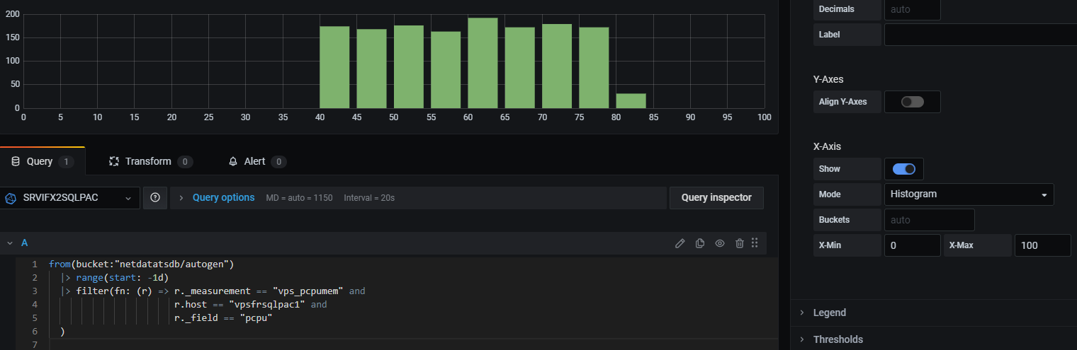
In Grafana, same methodology, the query source without histogram function call is used.
Computed columns - map
Computed columns are created with map function. map function is usually called after a join or a pivot operation.
In the example below, vps_space measurement stores two fields per point : used space (used) and available space (available).
In the final result set, we want to compute the space used percentage in a column named pctspace :
from(bucket: "netdatatsdb/autogen") |> range(start: -1d) |> filter(fn: (r) => r._measurement == "vps_space" and r.host == "vpsfrsqlpac1" and (r._field == "used" or r._field == "available") ) |> pivot( rowKey:["_time"], columnKey: ["_field"], valueColumn: "_value" ) |> map(fn: (r) => ({ r with pctspace: (r.used / (r.used + r.available)) * 100.0 })) |> keep(columns: ["_time", "pctspace"])_time:time pctspace:float ------------------------------ ---------------------------- 2021-03-01T17:51:47.437958334Z 73.84712268752916 2021-03-01T17:52:47.900410821Z 73.84713257521788 2021-03-01T17:53:48.389130505Z 73.8471523505953
The with operator is very important when calling map function.
In the default basic syntax (without the with operator),
columns that are not part of the input table’s group key (_time, _start, _stop…)
and not explicitly mapped are removed :
|> map(fn: (r) => ({ pctspace: (r.used / (r.used + r.available)) * 100.0 }))Table: keys: [] pctspace:float ---------------------------- 73.84734021668079 73.84734021668079
The with operator updates a column if it already exists, creates a new column if it doesn’t exist,
and includes all existing columns in the output table.
Cross computed columns
Computed columns referencing computed columns can not be defined in one unique map function call :
|> map(fn: (r) => ({ r with totalspace: r.used + r.available, pctspace: (r.used / r.totalspace) * 100.0 })) |> keep(columns: ["_time", "used", "totalspace","pctspace"])_time:time pctspace:float totalspace:float used:float ------------------------------ ---------------------------- ---------------------------- ---------------------------- 2021-03-02T18:33:36.041221773Z 40454348 29889216 2021-03-02T18:34:36.532166008Z 40454348 29889220
In this specific context, map function must be called sequentially :
|> map(fn: (r) => ({ r with totalspace: r.used + r.available })) |> map(fn: (r) => ({ r with pctspace: (r.used / r.totalspace) * 100.0 })) |> keep(columns: ["_time", "used", "totalspace","pctspace"])_time:time pctspace:float totalspace:float used:float ------------------------------ ---------------------------- ---------------------------- ---------------------------- 2021-03-02T18:33:36.041221773Z 73.88386533877645 40454348 29889236 2021-03-02T18:34:36.532166008Z 73.88388511415386 40454348 29889244
Conditions, exists
Conditions can be defined in map function and the exists operator is available :
import "math" … |> map(fn: (r) => ({ r with totalspace: r.used + r.available })) |> map(fn: (r) => ({ r with pctspace: (r.used / r.totalspace) * 100.0 })) |> aggregateWindow(every: 1m, fn: mean, column: "pctspace") |> map(fn: (r) => ({ r with pctspace: if exists r.pctspace then "${string(v: math.round(x: r.pctspace) )} %" else "N/A" })) |> keep(columns: ["_time", "used","pctspace"])_time:time pctspace:string ------------------------------ ---------------------- 2021-03-02T14:35:00.000000000Z 74 % 2021-03-02T14:36:00.000000000Z N/A
Custom aggregate functions - reduce
mean, max, min, sum, count… Flux functions are good shortcuts to aggregates,
but unfortunately only one aggregate can be returned.
from(bucket: "netdatatsdb/autogen") |> range(start: -1d) |> filter(fn: (r) => r._measurement == "vps_space" and r.host == "vpsfrsqlpac1" and (r._field == "used" or r._field == "available") ) |> pivot( rowKey:["_time"], columnKey: ["_field"], valueColumn: "_value" ) |> count(column: "used")used:int -------------------------- 1428
Multiple custom aggregate results can be extracted using reduce function
which returns a unique row storing the aggregates with no _time column.
from(bucket: "netdatatsdb/autogen") |> range(start: -1d) |> filter(fn: (r) => r._measurement == "vps_space" and r.host == "vpsfrsqlpac1" and (r._field == "used" or r._field == "available") ) |> pivot( rowKey:["_time"], columnKey: ["_field"], valueColumn: "_value" ) |> map(fn: (r) => ({ r with totalspace: r.used + r.available })) |> map(fn: (r) => ({ r with pctspace: (r.used / r.totalspace) * 100.0 })) |> reduce(fn: (r, accumulator) => ( { count: accumulator.count + 1, max: if r.pctspace > accumulator.max then r.pctspace else accumulator.max }), identity: {count: 0, max: 0.0} ) |> keep(columns: ["count","max"])count:int max:float ---------------------------- ---------------------------- 1428 73.93648761809237
identity defines the initial values as well as the data types (0 for an integer, 0.0 for a float).
Like map function, conditions and exists operator are allowed.
One may comment : what a stupid example ! The reduce function computes aggregates available
with native Flux functions, why reinventing the wheel ?
The reduce function indeed should be used for custom aggregates computations for which no native function exists.
The above example can be rewritten using native functions count and max, a join is performed :
dataspace = from(bucket: "netdatatsdb/autogen") |> range(start: -1d) … datacnt = dataspace |> count(column:"pctspace") |> rename(columns: {"pctspace": "count"}) datamax = dataspace |> max(column:"pctspace") |> rename(columns: {"pctspace": "max"}) join( tables: {cnt: datacnt, max: datamax}, on: ["_measurement"] ) |> keep(columns: ["count", "max"]) |> yield()count:int max:float -------------------------- ---------------------------- 1428 73.93870246036347
The above example would have been the following InfluxQL query with a subquery :
SELECT count(pctspace), max(pctspace)
FROM (SELECT (used / (used + available)) * 100 as pctspace
      FROM "netdatatsdb.autogen.vps_space"
      WHERE (host='vpsfrsqlpac1' and time > now() -1d)
)
Significant calendar functions enhancements
hourSelection
Selecting specified hours of the day was not possible using InfluxQL. Flux language supports DatePart-like queries with
the function hourSelection returning only data with time values in a specified hour range.
from(bucket: "netdatatsdb/autogen")
  |> range(start: -72h)
  |> filter(fn: (r) => r._measurement == "vps_pcpumem" and
                       r.host == "vpsfrsqlpac1" and
                       r._field == "pcpu"
  )
  |> hourSelection(start: 8, stop: 18)
  |> aggregateWindow(every: 1h, fn: mean)
Windowing data by month(s) and year(s)
Flux language supports windowing data by calendar months (mo) and years (yr) : 1mo, 3mo, 1yr…
This feature was not either possible with InfluxQL. Useful for producing KPI (Key Performance Indicators) per months, quarters, semesters, years.
|> aggregateWindow(every: 1mo, fn: mean)